Integrated Decision-Making Based on OLAP
OLAP systems allow flexible and dynamic questions to be asked of big data. By combining OLAP with multicriteria decision-making techniques, we can allow business executives to incorporate insights from real-world data into the systematic evaluation of different business options. This improves the quality of complex decisions and leads to better business outcomes with the same resources.
Application
Description of the case study
Issues related to the Green Supply Chain Management at the level of mining activities have serious social–environmental consequences and underlying economic implications. In this illustrative example linked to the field of green logistics, potential itineraries for the transport of chemicals in Casablanca industrial region (see Fig. 6) are assessed and classified for a sustainability objective. It examines several itineraries and controls their evolution during a period of time beginning from 2000 to 2013, according to several evaluation criteria as shown in Fig. 7, describing the hierarchical structure of this problem.

Itineraries of the industrial region of Casablanca

The hierarchical structure of the problem
However, achieving this objective is often complicated and requires consideration of tradeoffs between social–political, environmental and economic impacts. Moreover, the different types of data included in the decision-making process can be of a certain, uncertain, quantitative or qualitative nature, leading organizations to make decisions in important conditions of uncertainty, causing unexpected results. It is therefore necessary to look for decision support tools with high analytic capacity to meet certain characteristics and specificities of this type of problems, which we quote as follows: conflict of objectives; comparison of several possible actions according to several criteria and objectives; contradiction of criteria; qualitative and quantitative criteria; scalable and temporal aspects of certain criteria; ambiguity of preferences; and subjectivity of judgments of decision makers. All these situations merely highlight the complex and multicriteria aspects of this type of problems.
Analysis and results
Criteria evaluation phase: AMCD interface
The criteria presented in Fig. 7 are segmented according to an MDX query executed at the OLAP server, allowing to view in descending order all the evaluation criteria related to the choice of itineraries. This segmentation aims to simplify the selection of these criteria and consider only those with a high final score. In this context, the evaluation of these criteria via the AMCD interface is carried out according to six complementary steps as illustrated in Fig. 8. The first step consists in specifying the number of criteria to be considered in the evaluation. This is used by the AMCD interface to generate the comparison matrix corresponding to the number of criteria already specified.

Choice of the number of evaluation criteria (step 1)
At the beginning of the evaluation, according to the number of criteria set by decision makers using the AMCD interface (step 1 presented in Fig. 8), the criteria are numbered as follows: C1, C2, C3… and are directly modified by the decision makers (DM1, DM2, DM3), as illustrated in Fig. 9.

Appreciations of the criteria by the decision-making group
The role of decision makers is to complete the criteria evaluation matrix by their assessments for each criterion in relation to the others (Fig. 9). These qualitative assessments are based on linguistic variables (Table 2) representing the relative importance of paired elements, which are then transformed to fuzzy triangular numbers.
| Linguistic variables | Fuzzy numbers | TFN scales |
| Very good (VG) | \(\tilde{9}\) | (7, 9, 9) |
| Good (Gd) | \(\tilde{7}\) | (5, 7, 9) |
| Preferable (P) | \(\tilde{5}\) | (3, 5, 7) |
| Weak advantage (WA) | \(\tilde{3}\) | (1, 3, 5) |
| Equal (EQ) | \(\tilde{1}\) | (1, 1, 1) |
| Less WA | \(\tilde{3}^{-1}\) | (1/5, 1/3, 1) |
| Less P | \(\tilde{5}^{-1}\) | (1/7, 1/5, 1/3) |
| Less G | \(\tilde{7}^{-1}\) | (1/9, 1/7, 1/5) |
| Less VG | \(\tilde{9}^{-1}\) | (1/9, 1/9, 1/7) |
The reason for using these fuzzy numbers is that they are intuitively easy to use for capturing the vagueness and ambiguity of the language assessments provided by the decision group.
After finalizing the evaluation matrix by the linguistic appreciations of the decision group, we transform this qualitative data into numerical ones via fuzzy triangular numbers, in order to aggregate them as shown in Fig. 10.
Transformation of linguistic data and aggregation of triangular numbers
The fourth step of the AMCD interface, as mentioned in Fig. 11, calculates the geometric mean based on the aggregation of the fuzzy triangular numbers already calculated in step 3 of Fig. 10.

Calculation of the geometric mean
Then, based on the geometric mean already obtained, we calculate the fuzzy weights of the criteria which are in the form of a triangular fuzzy number using Eqs. (6–7) of Appendix A as illustrated in Fig. 12.
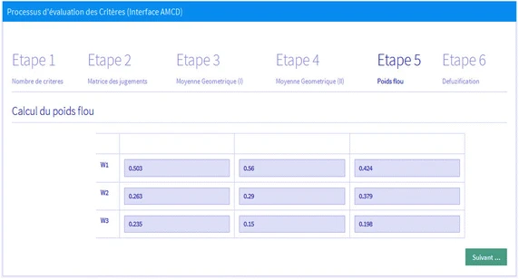
Fuzzy weight calculation
The final step of MCA process is to make the defuzzification of the fuzzy weight obtained in Fig. 12, using the gravity method applied via Eq. (8) of Appendix A. The final standardized weight resulting from this defuzzification is then obtained via Eq. (9) as shown in Fig. 13.

Calculation of the final standardized weight
Once the final standardized weight calculation (Fig. 13) of the main criteria has been completed and validated, the committee begins to calculate the subcriteria weights using the same interface and perform the final backup of all these weights in a CSV file. These weights are considered as inputs in upcoming alternatives evaluations (stage 2).
Identification and evaluation phase of alternatives (stage 1)
The proposed modeling to deal with the decision problem is presented in Appendix C using a multidimensional star schema. The implementation of this modeling integrates the design of an XML description file that describes the measurement axes (analysis axis) and the dimensions to consider before querying data through a client tool.
In this context, the second decision-making process that comes after completing the phase concerning the computation of the criteria weights is the evaluation of alternatives. Thus, the input data to be considered in step 1 of the alternative evaluation process are the selected criteria (without incorporating the weight of these criteria during this step), and the alternatives (itineraries) to be evaluated.
The first operation to be performed when analyzing the data in the alternatives evaluation phase is the exploration of the data cube through MDX queries, based on OLAP_MML interface editor provided in Fig. 14.

MDX query execution editor
The query execution editor allows users to create and execute instructions and scripts written in MDX language.
During the evaluation, the OLAP_MML interface offers the possibility to use the file containing the weights of the criteria calculated via the AMCD interface (see Fig. 15), when integrating the utility function (weighted sum) into the OLAP analysis process, as presented in the overall approach of our previous contributions.

Possibility of loading the CSV file containing the weights of the criteria
Nevertheless, our objective in this paper is to indirectly combine OLAP analysis with PROMETHEE as an outranking multicriteria method, which will be responsible for the consideration of the criteria weight when evaluating alternatives derived as output variables of the OLAP process. The reason to include the PROMETHEE method in the analysis process is to enable decision makers to better manage the limitations of the weighted sum method, primarily related to the problem of compensatory aggregation of actions.
Consequently, we execute MDX queries via the Mondrian OLAP server in order to illustrate the final results of the evaluation of all itineraries selected from the data cube as presented in Fig. 16, exploring the decision elements (criteria and actions) via the Jpivot interface of Mondrian OLAP server (the Mondrian/JPivot couple is available in the following suites: Pentaho Community Edition, JasperSoft, and SpagoBI).

Exploring decision elements via the Jpivot interface of OLAP Mondrian server
Figure 17 shows the result of using MDX queries through the OLAP_MML application in order to provide decision makers with a list of alternatives ranked by importance. These alternatives result from the aggregation of the values of the criteria versus the alternatives during the period 2000–2013.

MDX query for the analysis of potential itineraries
Based on the evaluation and analysis results presented in Fig. 17, 'itinerary-Ref013' is the most appropriate one followed by 'itinerary-Ref009' as the second choice, then 'itinerary-Ref007,' 'itinerary-Ref011,' …, until the last itinerary. The objective is to make a primary segmentation of the potential itineraries provided by OLAP analysis, and to consider them as input variables at the level of multicriteria analysis process proposed in the alternatives assessment phase (step 2).
Final evaluation phase of alternatives (stage 2)
The aim of this part is to analyze and evaluate a list of alternatives consisting of the first four itineraries resulting from the ranking provided by OLAP analysis process, based on the principle of the PROMETHEE method as a multicriteria decision-making aid method. This evaluation aims to integrate the importance weights assigned to the criteria in the MCA process in order to assist decision makers in choosing the best possible itinerary for the transport of chemicals in the industrial region of Casablanca.
To achieve this goal, we have used the Visual Promethee program which is an easy and practical multicriteria analysis program. It allows evaluating and ranking the alternatives, using the methodological approach of the PROMETHEE method to which the algorithm is presented in the Appendix B.
The decision makers' preferences for the evaluation of alternatives with respect to all the specified criteria will be made using linguistic scales for evaluation (Fig. 18 and Table 3).

Linguistic scales for evaluation
| Linguistic variables | Fuzzy triangular scale |
| Good (G) | (0.80, 1, 1) |
| Preferable (P) | (0.80, 1, 1(0.65, 0.80, 1) |
| Medium preference (MP) | (0.50, 0.65, 0.80) |
| Neutral (N) | (0.30, 0.50, 0.65) |
| Less G (L.G) | (0. 15, 0.30, 0.50) |
| Less P (L.P) | (0, 0. 15, 0.30) |
| Less MP (L.MP) | (0, 0, 0.15) |
In the same context, the V-shape preference function (see Fig. 19 and Appendix B – step 2) was selected by setting the value of the "P" parameter of this function to 2 for all selected criteria as shown in Table 4 and Fig. 20.

Fonctions de préférences de la méthode PROMETHEE
| Critères | EnC1 | EnC2 | SC1 | SC2 | EC1 | EC2 |
| Fct. Préference | V-shape | V-shape | V-shape | V-shape | V-shape | V-shape |
| Préférence (P) | 2 | 2 | 2 | 2 | 2 | 2 |
| Max/Min | Max | Max | Max | Min | Min | Max |
| Weight | 0.585 | 0.129 | 0.134 | 0.059 | 0.081 | 0.012 |
| tinerary-Ref013 | P | N | P | L.G | MP | L.MP |
| Itinerary-Ref009 | L.G | N | MP | P | L.P | MP |
| Itinerary-Ref007 | G | N | MP | MP | L | L.P |
| Itinerary-Ref011 | MP | L.G | L.P | N | MP | N |

Alternative evaluation matrix using Visual Promethee features
The geometrical analysis for interactive aid (GAIA) integrated in Visual Promethee program is used as a visualization method complementing the PROMETHEE ranking methodology, which will help to display graphically the relative position of itineraries in terms of contributions to the selected criteria (Fig. 21).

GAIA plan generated by Visual PROMETHEE
During this analysis, the criteria are represented by vectors, and the alternatives, by points as shown in Fig. 21. Additionally, the conflicting criteria appear clearly in the GAIA plane visualization. Criteria vectors that express similar preferences are oriented in the same direction, while conflicting criteria are pointing in opposite directions.
To sum up, the positive flow, negative flow and net outranking flow allowing to provide the final ranking of itineraries are obtained as shown in Fig. 22. The results obtained at this level may be sufficient, taking into consideration the objective of the decision.

Final result of net outranking flow
As shown in Fig. 22, the final evaluation of the most appropriate itineraries is provided. Indeed, each itinerary has its relative score calculated on the basis of the contribution of the weights of the selected criteria. Therefore, the most suitable itinerary is the one with the highest net outranking flow according to the final ranking shown in Fig. 22, which shows that the preferred itinerary is "itinerary-Ref007" with a net flow of 0.0948, followed by "itinerary-Ref013" (0.0889) and "itinerary-Ref011" (−0.0424) till the last preferred itinerary "itinerary-Ref009" (−0.1412).